Nearest Neighbor Networks
Welcome to NNN - we hope you find our software useful! NNN is
licensed under the
Creative
Commons Attributions 2.5 license, which means you can use it for
pretty much anything as long as you cite us. The relevant
publication is:
Huttenhower, C., Flamholz, A., Landis, J., Sahi, S., Myers, C.,
Olszewski, K., Hibbs, M., Siemers, N., Troyanskaya, O.,
Coller, H., "Nearest Neighbor Networks: Clustering Expression
Data Based on Gene Neighborhoods", BMC Bioinformatics 8:250,
2007
You can find more information about the NNN algorithm and its
performance in this paper, or you can check out the labs involved
in its creation:
Now, on to the good part...
Table of Contents
-
I just want to cluster genes!
- java.lang.OutOfMemoryError
-
Graphical interface
- Main panel
- Advanced options
- Command line interface
-
Input and output formats
- Inputs
- Outputs
- Source code
- Version history
I just want to cluster genes!
If you just want to get up and running with NNN, you need two
things:
- The NNN implementation, which can be downloaded
here.
- A PCL file containing the expression data you'd like to cluster.
A general overview of the PCL format can be found
here.
NNN is fairly generous in its parsing of PCL files; specifically,
it will ignore an EWEIGHT row if present (but it doesn't care if
there's no EWEIGHT row), and it will attempt to guess the number
of initial non-data columns (in other words, in addition to the
first ID column identifying your genes, you can include any number
of labeling columns such as NAME, GWEIGHT, and so forth). Missing
values will be handled correctly, but it is recommended that you
first filter and/or
impute missing data for better clustering performance.
When you start up NNN, you should see the following interface:
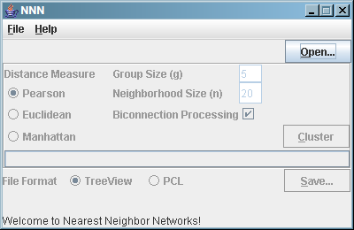 To cluster your data:
- Click the "Open" button and browse to your PCL file.
- Adjust the four options (distance measure, clique size g,
neighborhood size n, and biconnection processing) to best suit
your data set.
- We recommend the default settings for the "average"
microarray data set (Pearson, 5, 20, and yes), but
varying the neighborhood size can improve performance
substantially on particularly small (fewer conditions)
or large (more conditions) data sets.
- Clique sizes greater than six will take a very long
time to run, and they don't generally provide much
benefit!
- Turning biconnection processing off is basically never
useful.
- If you have a data set containing a very large number of
genes (e.g. human data), see the
advanced options
below for some tips on improving performance.
- Click the "Cluster" button and keep an eye on the progress bar!
The initial 2/3 are the slowest; the last 1/3 is just
biconnection processing (if selected), which is fast.
- Once your clustering is ready, you can save in either TreeView
or PCL formats.
- The TreeView format saves a CDT/GTR file pair
appropriate for viewing in
Java
TreeView. This is the recommended format for human
readable output.
- The PCL format saves a duplicate of the input PCL file
with a single additional column added, "Networks",
identifying the cluster(s) (if any) to which each gene
was assigned. This is the recommended format for
computer readable output.
If you made it this far successfully, congratulations - you've got
Nearest Neighbor Networks! If the output doesn't quite meet your
expectations, fret not - see below for additional options that can
be manipulated to further improve clustering performance.
java.lang.OutOfMemoryError
Under certain circumstances (generally only when using the command
line interface), you might get a java.lang.OutOfMemoryError
error while using NNN. This is spectacularly easy to fix, however;
from the command line (either the Command Prompt on Windows,
Terminal on Mac OS, or your console of choice on Linux), start up
NNN using the command:
java -Xmx1024m -jar nnn<your version number here>.jar
You can substitute larger numbers than 1024 if you have lots of
free memory sitting around; well-behaved JVMs won't use the extra
memory unless they need it.
Graphical interface
Main panel
The elements of the default graphical interface are (hopefully)
fairly self-explanatory (at least if you've read our paper!) In
order, these are:
- Distance Measure. Three options are included by default
for measuring gene pair similarity: Pearson correlation,
Euclidean distance (L2 norm), and Manhattan distance (L1 norm).
If you're interested in seeing more distance measures,
let us know!
- Group Size (g). As described in the paper, this is the
clique size NNN will search for in its preliminary interaction
network while combining overlapping cliques into clusters.
Values below two don't make much sense, and values above six
will be slooooow for any reasonably sized data set. In general,
there's no huge benefit in increasing g above five, and
decreasing it will only hurt performance.
- Neighborhood Size (n). As described in the paper, this
is the number of nearest neighbors NNN will use while forming
its preliminary mutual nearest neighbor interaction network.
This is the parameter most relevant to performance tuning, and
it is directly related to the number of conditions in your data
set. Data sets with more conditions might want to use a larger
n, but using too large of a value will result in overlarge
clusters. Conversely, too small of an n will generate lots of
tiny clusters. Larger values of n will make things somewhat
slower, but not critically so in general.
- Biconnection Processing. If this option is activated,
NNN will split clusters containing cut-vertices into multiple
connected components. In other words, this removes hubs from
the clusters that may be joining clusters that are otherwise
functionally unrelated. It's a fast process, so there's rarely
any reason to deactivate it.
- The progress bar and status bar indicate, well,
the progress and status of clustering, respectively. The
progress bar will advance during a clustering run, and the
status bar will display various text that's potentially
relevant to the status of data input and clustering
results.
Advanced options
If you activated the "Advanced" checkbox under the "File" menu,
NNN displays a few additional options:
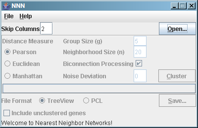 These extra options are:
- Skip Columns. If NNN fails to correctly guess the
column in which the expression data begins in your PCL file,
you can force it to skip a specific number of columns. This
is the number of columns to skip after the first column,
which must contain unique gene IDs. For example, if your
column headers were GID, NAME, GWEIGHT, Time point 1, Time point
2, and so forth, the skip value should be two (to account for
NAME and GWEIGHT).
- Noise Deviation. In data
sets containing a large number of genes, it is sometimes
difficult to balance the neighborhood size to retrieve many
medium sized clusters (rather than a few huge ones or a bunch of
tiny ones). NNN offers the option of using a very basic
simulated annealing approach by adding some noise to the initial
neighborhood distance calculations, in effect "jittering apart"
the nearest neighbors that aren't particularly tight (and thus
probably not functionally meaningful) and breaking up overlarge
clusters. This parameter controls the standard deviation of
normally distributed random noise to be added to the distance
calculations - which means it should be small! A deviation of
0.05 or 0.1 is generally sufficient for Pearson correlation,
while an appropriate value for other measures will depend on
the characteristics of your data.
- Include unclustered genes. By default, when saving a
TreeView file, NNN only includes genes that have been included
in at least one NNN cluster. If this option is enabled, all
genes will be included in the TreeView file (although only NNN
clusters will be colored). Activating this option can increase
save times (since a full hierarchical clustering needs to be
calculated). The PCL output format always includes all
genes.
Command line interface
In addition to the graphical interface, NNN has a command line
interface that 95% of its users probably won't care about. But if
you're interested in getting into the nitty gritty of NNN's
capabilities, read on! Using the command line, you can obtain
additional output formats or provide additional input to influence
NNN's clustering behavior.
If you call NNN with no command line arguments, you'll get the
graphical interface described above. But if you provide any
command line arguments, the console-based version will run instead.
In particular, providing the "-h" argument produces the following
information:
 -g N       : Group size (5)
              0 produces NN distance only
 -n N       : Minimum neighborhood size (20)
 -N N       : Maximum neighborhood size (n)
 -e N       : Neighborhood size step (5)

 -m MEASURE : Distance measure (Pearson)
              Peason, Euclidean, Manhattan
 -d N       : Deviation of added Gaussian noise (0)
 -z FILE    : Precalculated distance file

 -s         : Separate biconnected components (true)
 -l         : Remove overlarge networks (true)
 -u         : Hierarchically cluster genes that aren't clustered by NNN (false)

 -i FILE    : Input file (standard in)
 -k N       : Columns to skip after the initial gene ID in input PCL (auto)
 -o FILE    : Output file (standard out)
 -t FILE    : Produce a TreeView CDT/GTR (none)

 -p FILE    : TFBS profile PCL file (none)
 -K N       : Columns to skip after the initial gene ID in profile PCL (auto)
 -b N       : Weight of TFBS profiles (0)
Many of these options are available through the GUI, and the default
behavior of the command line interface is essentially identical to
the default behavior of the GUI (default values are indicated in
parentheses). However, there are two significantly different
paradigms supported by the command line:
- The command line can run NNN several times with a fixed clique
size g but while varying the neighborhood size n. This is
much more efficient than running NNN separately multiple times!
This is the technique we used to generate many of the figures
in the paper.
- NNN can incorporate additional information from TFBS profiles
into its distance calculations. We've never found this to be
particularly useful, but it's still in the interface in case
you're interested.
There are a lot of options there, so let's try to explain them:
- -g, group size (5). This is identical to the graphical
group size option. The one difference is that if you provide
a group size of zero, the command line interface will output
for each gene pair A and B the smallest neighborhood (within the
-n to -N range; see below) within which A and B are mutual
nearest neighbors. For example, suppose you have the following
genes and nearest neighborhoods (sorted from closest to
furthest):
- A: B, C, D
- B: A, D, C
- C: D, A, B
- D: C, B, A
Then with -g set to zero, NNN will produce:
A B 1
A C 2
A D 3
B C 3
B D 2
C D 1
This measure can be treated as sort of a distance metric
(larger values mean the genes are less similar), but none of
our experiments with it showed it to be very useful. Let us
know if you make it work!
- -n, minimum neighborhood size (20). This flag is
essentially identical to the GUI neighborhood size parameter,
unless you also provide a maximum neighborhood size -N.
- -N, maximum neighborhood size (n). By default, a
single neighborhood size is used (as it is in the GUI), so -N
will equal -n. If you provide a -N larger than -n, NNN will
cluster your genes at each neighborhood size between -n and
-N in steps of -e (the increment size). The output will then
be not a single clustering, but for each gene pair, the
minimum neighborhood size at which they clustered together.
For example, -n = 1, -N = 3, and -e = 1 will produce the same
output as shown above for -g = 0. This is a useful way to
perform many clusterings efficiently.
- -e, neighborhood size step (5). This is the increment
by which NNN will step between -n and -N when performing
multiple clusterings. Any value between one and five is
useful, depending on how patient you are.
- -m, distance measure (Pearson). Identical to the GUI
option of the same name.
- -d, deviation of added Gaussian noise (0). Identical to
the GUI option of the same name.
- -z, precalculated distance file. The command line
version of NNN has the ability to read in precalculated
distances rather than calculating Pearson/Euclidean/etc.
measures on the fly. This can be useful for speeding things
up (since you only need to do the calculation once and store
it) or for clustering based on a distance measure of your own.
However, the file format in which the precalculated distances
are stored is a little arcane; if you're interested in this,
see below for a discussion of the source
code.
- -s, separate biconnected components (true). Identical to
the GUI option of the same name.
- -l, remove overlarge networks (true). When set, NNN
will avoid removing clusters containing >50% of the input
genes. Removing these is basically always the right thing to
do, so don't set this flag unless you're really sure you want
weird output!
- -u, include unclustered genes (false). Identical to the
advanced GUI option of the same name.
- -i, input file (standard in). The input PCL file to
cluster, read from standard input by default. All of the same
comments apply as to the GUI version.
- -k, skip columns (auto). Identical to the GUI option of
the same name.
- -o, output file (standard out). The output CDT or PCL
file; PCL output is written to standard output by default. All
of the same comments apply as to the GUI version.
- -t, produce TreeView output (none). The default output
format from the command line is a PCL with the "Networks"
column added, but it can produce a TreeView .cdt/.gtr file pair
if requested (which is the GUI's default). If a filename is
provided for -t, either as a base name or a .cdt, the
appropriate .cdt/.gtr pair will be generated (in addition to
PCL output to standard output or -o).
- -p, TFBS profile file (none). The command line version
of NNN can incorporate TFBS profile similarities into its
distance measures in a fairly naive way. TFBS profiles are
provided in exactly the same format as coexpression data, but
each column should represent one TFBS, and each gene's score
in that column represents some sort of strength of association
(upstream count, PWM matches, etc.) Distances between TFBS
profiles are then incorporated into each gene pair's distance
using the -b parameter (below).
- -K, TFBS skip columns (auto). Same as the -k flag, but
applies to the TFBS input file instead.
- -b, weight of TFBS profiles (0). If TFBS profiles are
given, distances between gene pairs are calculated as:
d'(g1, g2) = b * d(p(g1), p(g2)) + ( 1 - b ) * d(g1, g2)
where d is the original distance measure, g1
and g2 are two genes, p(g) is the TFBS
profile of a gene, and b is the weight specified by
-b. In other words, if -b is zero, TFBS profiles aren't used;
if -b is one, coexpression isn't used. Anything in between
weights the two factors accordingly.
Input and output formats
Inputs
NNN's primary input format is the
PCL
file, a standard tab-separated tabular microarray data format.
In brief, the first row contains headers labeling each column. The
second row may contain an EWEIGHT line listing relative weights of
individual conditions (which NNN ignores), or it may contain the
first data record. Each subsequent row represents a single gene or
probe's data record, consisting of an initial unique ID, zero or
more label columns (such as NAME, GWEIGHT, and so forth), and one
or more data columns (individual microarray conditions).
NNN will attempt to guess the correct number of label columns to
skip; in general, PCL files of the form:
GID NAME GWEIGHT Condition 1 Condition 2 ...
and PCL files of the form:
GID NAME Custom label 1 Custom label 2 GWEIGHT Condition 1 Condition 2 ...
and PCL files of the form:
GID Condition 1 Condition 2 ...
will all work, so long as the custom label values aren't all numbers
(since that will trick NNN's guesser into thinking they're
expression values). NNN should deal equally well with PCL files
resulting from one- or two-channel arrays, although you should
ensure that one-channel array values are log transformed before
clustering (this is a semi-standard practice anyhow).
NNN will correctly parse missing values in its input PCLs, although
too many missing values may degrade clustering performance. We
recommend removing any gene with too many missing values (>30% of
the conditions) and
imputing any that remain.
Finally, NNN uses a custom DAT or DAB format for
advanced users wishing to provide precalculated distances through
the command line interface. For more information, see the
command line and source
code sections below.
Outputs
The NNN GUI and command line interfaces both provide two main
output formats. The graphical interface defaults to a .cdt/.gtr
file pair suitable for viewing in
Java TreeView. The
command line interface defaults to a single .pcl file annotated with
one new column, "Networks", indicating which clusters (if any) each
gene was placed into. Both of these formats are standards that are
described in detail elsewhere:
The command line interface also offers a pairwise output format for
advanced users of the form:
GENE1	GENE2	SCORE
GENE1	GENE3	SCORE
GENE2	GENE3	SCORE
and so forth. Each row contains a pair of gene identifiers and some
score (distance, neighborhood size, etc.) between them. Each line
is unique (i.e. each gene pair is contained only once in the file),
and each column is tab separated. This format is sometimes referred
to as a .dat file, the textual version of a .dab file (see the
source section for details).
Source code
NNN is provided with source code containing fairly extensive
JavaDoc and non-JavaDoc comments, so I won't spend much time on it
here. However, as an overview, the code consists of three main
pieces:
- The Args4J library,
which handles all of the command line argument processing.
Thanks, Args4J!
- The edu.princeton.cs.troyanskaya.lib package, which
handles all of the basic functionality not specific to NNN
clustering (PCL parsing, distance functions, storing scores,
etc.)
- The edu.princeton.molbio.koller.nnn package, which
contains everything specific to NNN (nearest neighbor
calculations, clique finding, cut-vertex finding, etc.)
The troyanskaya.lib package in particular contains
several classes which may be of general use, including:
- CCompactMatrix and CDac, a pair of classes
which store discrete pairwise scores in an extremely memory
efficient manner (sub-byte alignment). This is what makes it
possible to store all ~800M pairwise human scores in memory at
once.
- CHalfMatrix and CDat, a pair of classes
storing continuous pairwise scores in a less memory efficient
manner (but with better performance speed-wise). This is what
you should look at if you're interested in dealing with
precomputed distance.
- CClustHierarchical, a fairly simple hierarchical
clustering implementation.
Feel free to use any of these classes in your own applications,
modified or unmodified, so long as you cite us as per the
Creative
Commons Attributions 2.5 license. Thanks for being interested
enough in NNN to make it through all of these details, and happy
clustering!
Version history
- 0.9, 11-03-06
Initial release to reviewers.
- 0.91, 02-07-07
Minor documentation and CLI bug fixes.
- 0.92, 05-24-07
Bug fix addressing malformed values in input PCLs.
- 1.00, 07-30-07
No change from 0.92, version at time of publication.
- 1.01, 01-25-08
Huge hierarchical clustering speedup due to Mike Miller, added
joint PCL and CDT output.